Chemical
Equilibrium
1.
Introduction
The topic of chemical equilibrium follows logically from the topic of chemical kinetics. In looking at kinetics, we often studied the initial rates of reactions. We did this to minimize the importance of any possible reverse reaction, so we could focus on the forward reaction only. In studying chemical equilibrium, we consider both the forward and reverse directions of the reaction.
To
develop the concept of chemical equilibrium, let us consider a generic reaction
in which some arbitrary substances A and B react with each other to form some
other substances C and D. We can use
small letters a, b, c and d to indicate the coefficients of these substances in
the balanced equation. We can then
write the following equilibrium reaction:
aA +
bB <-----> cC
+ dD [Eq. 1]
In
equation 1, the double arrow indicates that the reaction is reversible – that
is, that once C and D have been formed, they can react with each other to
re-form the original substances A and B.
Suppose
we have a closed reaction vessel in which we start out with only substances A
and B, with no C or D initially present.
If A and B molecules collide with each other in the correct orientation
and with sufficient energy (activation energy or greater), they can react to
form C and D. One of the things that
governs reaction rate is collision frequency, which in turn, is proportional to
concentration. The concentrations of A
and B are highest at the beginning of the reaction, and decrease as A and B are
consumed in the forward reaction.
Therefore, the forward reaction rate will have its maximum value at the
beginning of the reaction (“time zero”).
The forward rate will decrease as the reaction proceeds, because A and B
are being removed and replaced with C and D.
The rate of the reverse reaction is initially zero, because no C and D
are initially present. If no C and D
are present, there can be no collisions between C and D molecules. Therefore, the collision frequency is zero, and
so, the reverse reaction rate is also zero.
However, as the forward reaction produces C and D, their concentrations
begin to increase. With C and D now
present, collisions between C and D molecules begin to occur, and a reverse
reaction is observed. As time goes on,
the concentrations of C and D increase as these substances continue to be
formed by the forward reaction. This
increasing concentration of C and D causes the collision frequency (of C and D)
to increase, leading to a higher reverse reaction rate. At the same time, the forward reaction is
slowing down, because A and B are being removed from the container (by being
converted to C and D). The decreasing
concentrations of A and B lead to a lower collision frequency between A and B
molecules, and therefore, a lower forward reaction rate.
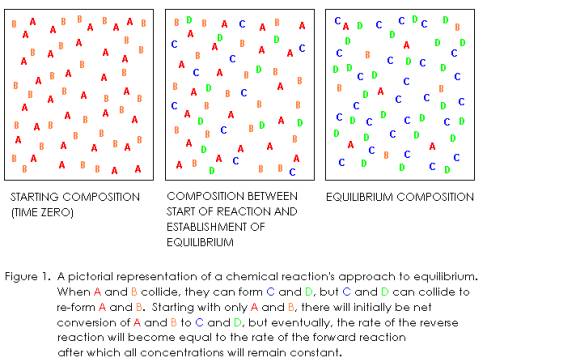
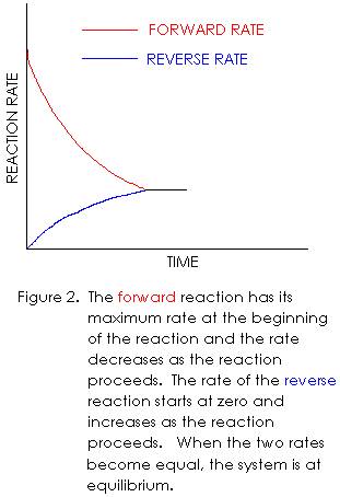
From
the above description, we see that the forward reaction has its maximum rate at
the beginning of the reaction, and the rate decreases as the reaction
occurs. We also see that the reverse
reaction rate starts out at zero, and increases as the reaction occurs. There will eventually come a time when the
forward and reverse reactions have the same rate. We call this condition chemical equilibrium. When equilibrium is reached, the
concentrations of all substances in the reaction (A, B, C, and D in this case)
remain constant. This is because the
forward and reverse reactions have exactly opposite effects. When they occur at the same rate, they
cancel each other’s results. The
forward reaction removes A and B from the container, while the reverse reaction
returns the A and B. Likewise, the
forward reaction forms substances C and D, while the reverse reaction removes
them.
Even
though the concentrations of all substances remain constant at equilibrium, the
forward and reverse reactions have not
stopped. For this reason, we say
chemical equilibrium is dynamic.
Students sometimes have the misconception that everything is stopped at
equilibrium, because equilibrium systems have no macroscopic change. In chemistry, however, things continue to
happen at the microscopic level, even though all macroscopically observable
properties remain constant.

2. Derivation of the Equilibrium Constant
2.1 An Elementary Reaction
Let
us return to the reaction we looked at in the introduction,
aA +
bB <-----> cC
+ dD [Eq. 1]
and
for the time being, assume it to be an elementary reaction. For an elementary reaction, we know that the
reaction orders must be the same as the coefficients in the balanced
equation. Because we are now looking at
both directions of reaction, we can
write a rate law for the forward reaction and
for the reverse reaction. We will use Rf
and kf to represent the forward rate and forward rate constant, and
we will use Rr and kr to represent the reverse rate and
reverse rate constant. The two rate
laws will have their usual form:
Rf = kf [A]a [B]b [Eq.
2]
Rr = kr [A]a [B]b [Eq.
3]
At
equilibrium, the forward rate and reverse rate will be equal, that is,
Rf = Rr [Eq.
4]
By
substituting equations 2 and 3 into equation 4, we obtain
kf [A]aeq [B]beq = kr [C]ceq [D]deq [Eq. 5]
In
equation 5, the subscript eq has been added to each concentration to remind us
that the equation only holds true when an equilibrium set of concentrations is
used. What we want to do now is gather
the rate constants on the left side of the equation, and the concentrations on
the right side. If we divide both sides
of equation 5 by kr we obtain
(kf / kr) [A]aeq [B]beq =
[C]ceq [D]deq [Eq. 6]
Then,
dividing both sides of equation 6 by [A]aeq [D]deq
gives
(kf / kr) =
[C]ceq [D]deq /
[A]aeq [B]beq [Eq. 7]
Notice
that the left hand side of equation 7 is just a ratio of two constants. Although rate constants are temperature
dependent (as given by the Arrhenius equation), they are independent of
concentration. If we assume the
equilibrium reaction occurs at constant temperature (as will usually be the
case in this course), the left hand side of equation 7 is a constant. The right hand side consists of a function
of concentrations, which can vary. The
subscript eq on all the concentrations reminds us that this apparent paradox is
not really a paradox at all. While the individual concentrations can vary, the
mathematical combination of these concentrations shown in equation 7 can not vary. Of course, in order for this to work, we must use a set of equilibrium concentrations. We could study 100 different equilibrium
mixtures of substances A, B, C, and D (at the same temperature, of course) and
find a different concentration of substance A in every one of them. Likewise, substances B, C, and D could each
have a different concentration in every equilibrium mixture we looked at. However, if we plugged the concentrations
into the right hand side of equation 7, we would find that we would get the
same number every time. That is, every
chemical reaction, written in a particular form, at a given temperature, has a
characteristic number that we call the equilibrium constant. When you plug the concentrations into the
right hand side of equation 7, if you don’t get that characteristic number, you
don’t have an equilibrium set of concentrations.
We
can write the left side of equation 7 as a single constant by noting that a
constant divided by a constant is just another constant. If we define the equilibrium constant KC
such that
KC = kf
/ kr [Eq.
8]
and
substitute equation 8 into equation 7, we have
KC =
[C]ceq [D]deq / [A]aeq
[B]beq [Eq.
9]
Equations
1 and 9, taken together, show us how to write the equilibrium constant
expression (sometimes called equilibrium law) for a chemical reaction. The form of the equilibrium constant (KC)
expression is a ratio of concentrations, with the substances that are on the
right hand side of the chemical equation appearing in the numerator, and the
substances that are on the left hand side of the chemical equation appearing in
the denominator. Each concentration is
raised to a power equal to its coefficient in the balanced equation.
The
equilibrium constant (KC) expression (equation 9) that was derived
in this section was based on the assumption that the equilibrium reaction was
an elementary reaction. It turns out,
however, that the equilibrium constant expression has the same form even if the
reaction is not elementary. To illustrate
this, we will look at an example of a non-elementary reaction in the next section.
2.2 A Non-elementary Reaction
In Section 2.1, we derived the equilibrium constant expression for an elementary reaction. To show why an equilibrium reaction has the same equilibrium constant expression even if it is not elementary, let’s consider the following non-elementary reaction:
2NO2(g) +
F2(g)
<-----> 2NO2F(g) [Eq. 10]
Experimentally,
it can be shown (using the method of initial rates, which we learned about in
our study of kinetics), that the rate law of the forward reaction is
Rf = kf [NO2] [F2] [Eq.
11]
Comparing
equations 10 and 11, we see that this reaction is definitely not
elementary. If the reaction was
elementary, the rate law would have to be second order in NO2,
because the coefficient of NO2 in the balanced equation is 2. However, experimental data shows the
reaction to be first order in NO2.
This is reflected by the exponent of 1 (understood and not shown) on [NO2]
in equation 11.
An elementary reaction is one that takes place in a single step, exactly as written. Since the chemical reaction represented by equation 10 is not elementary, it actually takes place in 2 or more simpler steps. Equation 10 is merely the net effect of the simpler steps. It is believed that this reaction occurs in two steps, as shown below:
Step
1: NO2(g) +
F2(g)
<-----> NO2F(g) +
F(g) [Eq. 12] (slow)
Step
2: NO2(g) +
F(g) <-----> NO2F(g) [Eq.
13] (fast)
Notice
that if we add the chemical equations that are shown as equations 12 and 13,
the result is identical to equation 10.
In adding equations 12 and 13, we cancel out the monatomic fluorine
atom, because it appears as both a reactant and a product. A species like this, that forms in one
reaction and is then used in another, is called a reaction intermediate. When a reaction intermediate appears in a
reaction mechanism, it cancels out when the individual steps of the mechanism
are added.
Often,
when a mechanism is proposed, it is a reasonable assumption that one of the
reactions is a lot slower than the others.
In the mechanism we are looking at right now, the first step is believed
to be slow because it generates an isolated fluorine atom. We know that elemental fluorine is normally
encountered as diatomic molecules, that is, F2. Because of their high reactivity, individual
fluorine atoms are unstable, and in most environments, will rapidly react with
something to form a more stable species.
Therefore, we predict that isolated fluorine atoms will be formed only
with difficulty (which means they will be slow to form) but that once formed,
they will rapidly react with something to form a more stable entity. For this reason, we label the first step
“slow” and the second step “fast”.
Now
consider the rate of the overall process, represented by equation 10. Since it is the overall result of steps 1
and 2 (equations 12 and 13) taken together, the overall process can not be
completed any faster than the slowest step can be completed. Therefore, step 1 (equation 12) sets the
rate of the overall process. The
individual steps within a proposed mechanism are, by assumption, elementary. If we believed any of the steps were not
elementary, we would break them down into additional steps, until only
elementary steps remained. Since
equation 12 sets the rate for the overall process, the rate law for the overall
reaction (equation 10) will be that of equation 12. Since equation 12 is taken to be elementary, the rate law for
that equation must have reaction orders that match the coefficients in the
equation. Therefore, equation 12
predicts that the reaction will be first order in both NO2 and F2,
in agreement with experimental data, and represented by equation 11. We can now understand why non-elementary
reactions do not need to have reaction orders that match the coefficients in
the balanced equation. It is because
the rate law is not set by the overall reaction, but instead, by one of the
steps in the mechanism – which need not have the same coefficients as those
that appear in the overall reaction.
Now
let us consider the reaction in equation 10 when it reaches equilibrium. What is its equilibrium constant? If we use the pattern developed in Section
2.1, we can write the following equilibrium constant expression to go with this
reaction:
2NO2(g) +
F2(g)
<-----> 2NO2F(g) [Eq. 10]
KC =
[NO2F]2eq / [NO2]2eq
[F2]eq [Eq.
14]
Of
course, one could criticize this equilibrium constant expression (equation 14)
because the pattern we made use of was derived for elementary reactions, and
the reaction in equation 10 is not elementary.
To address this criticism, let’s obtain the equilibrium constant
expression in a different way.
In
order for the overall reaction (equation 10) to be at equilibrium, each of its
individual steps must be at equilibrium.
If the reaction shown in equation 10 actually occurs in two steps, as
shown in equations 12 and 13, then the reactions in equations 12 and 13 must be
at equilibrium. Since these reactions
are assumed to be elementary, we can apply the pattern developed in Section 2.1
without the argument that might be raised if we tried to apply it directly to
the reaction in equation 10. Let us
refer to the equilibrium constant of step 1 (equation 12) as KC1 and
to the equilibrium constant of step 2 (equation 13) as KC2. We can then write the following:
NO2(g) +
F2(g)
<-----> NO2F(g) +
F(g) [Eq. 12]
KC1 =
[NO2F]eq [F]eq / [NO2]eq
[F2]eq [Eq.
15]
NO2(g) + F(g) <-----> NO2F(g) [Eq. 13]
KC2 =
[NO2F]eq / [NO2]eq [F]eq [Eq. 16]
Since
a constant multiplied by a constant is another constant, let’s investigate what
constant we get by multiplying KC1 by KC2.
KC1
. KC2 = (
[NO2F]eq [F]eq / [NO2]eq
[F2]eq ) .
( [NO2F]eq
/ [NO2]eq [F]eq )
= [NO2F]2eq
/ [NO2]2eq [F2]eq [Eq.
17]
Notice
that the final result of equation 17 is identical to the right hand side of
equation 14. We only need to define KC
as the product of KC1 and KC2, that is,
KC = KC1 . KC2 [Eq.
18]
to
completely reproduce equation 14.
Therefore, even though the reaction in equation 10 is not elementary, it
has the same equilibrium constant expression as it would have if it was
elementary. This result applies to all
non-elementary reactions. A
non-elementary reaction consists of 2 or more elementary reactions that take
place in sequence. If we add these
reactions together, we get the equation for the overall reaction. If we write equilibrium constant expressions
for each of these elementary steps and then multiply them together, we get the
same expression as we would have written if we had assumed the overall reaction
to be elementary in the first place.
Thus, the equilibrium constant expression for a chemical reaction can be
written by inspection, without knowing whether or not the reaction is
elementary.
One
other benefit we have obtained from this analysis is that we have seen that
when chemical reactions are added, their equilibrium constants are
multiplied. In the next section, we
will consider other ways we might alter chemical reactions, and the associated
changes we would need to make to the equilibrium constant.
3. Manipulating Chemical Equations
3.1 Adding Chemical Equations
We
saw in the last section that when
chemical reactions are added, their equilibrium constants are multiplied. This arose in our demonstration that
chemical reactions have the same equilibrium constant expressions whether or
not they are elementary. The reader is
referred back to Section 2.2 for proof of the italicized statement made in this
section.
3.2 Multiplying a Chemical Equation by a
Constant
When a chemical equation is
multiplied by a constant, the equilibrium constant is raised to that power. For example, if you multiply a chemical equation by 2, you square
its equilibrium constant. To see this,
let’s reconsider the equations
aA +
bB <-----> cC
+ dD [Eq. 1]
and
KC =
[C]ceq [D]deq / [A]aeq
[B]beq [Eq.
9]
If
we multiply the chemical equation in equation 1 by the constant n (where
usually n is either a whole number like 2, 3, 4 and so on, or a fraction like ½
or ¼), we have
naA +
nbB <-----> ncC
+ ndD [Eq. 19]
With
equation 1 re-written in the form seen in equation 19, we apply the pattern
seen in equation 9 to get
K’C =
[C]nceq [D]ndeq / [A]naeq
[B]nbeq [Eq.
20]
where
the “prime” mark has been added to distinguish the variable from the one in
equation 9. In equation 20, we notice
that every exponent contains n as a factor.
We can therefore pull out that common factor and write the following:
K’C = (
[C]ceq [D]deq / [A]aeq
[B]beq )n =
( KC )n [Eq. 21]
As equation
21 shows, the “new” equilibrium constant (K’C) is just the original
equilibrium constant (KC) raised to the power n. This proves the statement made in italics at
the beginning of this section.
3.3 Reversing the Direction of a Chemical
Reaction
When a chemical equation is
reversed, the equilibrium constant for the reversed equation is the reciprocal
of the equilibrium constant for the original equation. To see this, let us again consider equations 1 and 9.
aA +
bB <-----> cC
+ dD [Eq. 1]
KC =
[C]ceq [D]deq / [A]aeq
[B]beq [Eq.
9]
If
we reverse the direction of the reaction in equation 1, we have
cC +
dD <-----> aA
+ bB [Eq. 22]
and
applying to equation 22, the pattern depicted by equations 1 and 9, we have
K’C =
[A]aeq [B]beq / [C]ccq
[D]deq [Eq.
23]
Comparing
equations 9 and 23, we see that exchanging the numerator and denominator on the
right hand side of equation 9 gives the right hand side of equation 23. Therefore, one expression is just the
reciprocal of the other.
K’C = 1
/ KC = ( KC
)-1 [Eq.
24]
Looking
at the final expression on the right hand side of equation 24, and recalling
the principle developed in Section 3.2, we see that reversing the direction of a
chemical equation is mathematically equivalent to multiplying it by -1. When the original equation is reversed, its
equilibrium constant gets raised to the -1 power, and Section 3.2 shows that
multiplying a chemical equation by a constant raises the equilibrium constant
to that power.
4. Uses of the Equilibrium Constant
So far, we have defined what an equilibrium is, derived the equilibrium constant from scratch, and explored several of its properties. But other than an intellectual exercise, is the equilibrium constant good for anything? Most definitely! In this section, we explore several important uses of the equilibrium constant.
4.1 Predicting the Position of Equilibrium
Many chemical reactions have numerical values that are either very large or very small. For these reactions, the numerical value of the equilibrium constant tells us what distribution of reactants and products to expect at equilibrium. Another way to say this is that the equilibrium constant lets us predict the completeness of reaction. For example, consider the following chemical reaction and associated equilibrium constant:
2SO2(g) +
O2(g)
<-----> 2SO3(g) KC = 8.0 x 1035 [Eq. 25]
Because
the algebraic form of the equilibrium constant expression for this reaction
will be
KC =
[SO3]2eq / [SO2]2eq
[O2]eq [Eq.
26]
the
large numerical value of KC given in equation 25 tells us that the
concentration of SO3 must be much greater than that of SO2
and O2. In equation 26, the numerator
is obviously much larger than the denominator if the quotient is a number on
the order of 1035. If we
start with a stoichiometric mixture of SO2 and O2, we
expect essentially complete conversion into SO3. For example, if we mixed 2 moles of SO2
and 1 mole of O2, we would expect to find 2 moles of SO3
at equilibrium. The remaining SO2
and O2 in the equilibrium mixture would be so small it would not be
worth considering, and the amount of SO3 would be so close to 2
moles (actually just a very very very tiny amount less than 2 moles)
that we could consider it to be exactly equal to 2 moles. The important principle you should remember
from this is the following:
When
the equilibrium constant (KC) is a very large number, the
equilibrium very much favors the right hand side. A stoichiometric mixture of reactants is essentially 100%
converted into products. In this case,
we can use stoichiometry alone (no need to do an equilibrium calculation) to
predict the equilibrium composition of the chemical system, given the starting
composition.
Now consider the other extreme – a reaction with a very small equilibrium constant.
2HF(g) <-----> H2(g) + F2(g) KC
= 1 x 10-95 [Eq. 27]
The
algebraic form of the equilibrium constant expression for this reaction will be
KC = [H2]eq
[F2]eq / [HF]2eq [Eq.
28]
In
order for the ratio in equation 28 to produce the very small numerical value
seen in equation 27, the equilibrium concentration of HF must be very much
larger than that of H2 and F2.
That is, there is essentially no reaction. Almost all the original HF remains at equilibrium. Only a very very very tiny amount of
it was converted to H2 and F2. The concentration of H2 and F2 in the
equilibrium mixture is so small that it is not worth considering. The amount of HF removed by the reaction is
so small that we can consider the equilibrium amount of HF to be equal to the
original amount of HF. The important principle
you should remember from this is the following:
When
the equilibrium constant (KC) is a very small number, the
equilibrium very much favors the left hand side. The reactants have essentially no reaction, and no detectable
amount of product is formed. We can
approximate this as 0% reaction.
When
the equilibrium constant (KC) is neither very large nor very small,
there will be significant amounts of both reactants and products present in the
equilibrium mixture. As we will see
later, the equilibrium constant expression can be used to calculate the
equilibrium composition, given the starting composition. Reflecting on the results we have obtained
looking at the preceding two reactions, we note the following:
The
smaller the value of KC, the more the equilibrium favors the left
hand side of the chemical equation, and the larger the value of KC,
the more the equilibrium favors the right hand side. For extremely small values of KC, the extent of
reaction is approximately 0%, and for extremely large values of KC,
the extent of reaction is essentially 100%.
There
is not a clear-cut number where KC becomes “extremely large” or
“extremely small”, but it is usually safe to say that a double digit positive
power of 10 is “very large” and a double digit negative power of 10 is “very
small”.
4.2 Finding an Equilibrium Concentration
If we know all the equilibrium concentrations in a chemical system except one, we can find the remaining equilibrium concentration from the equilibrium constant expression. For example, consider the following problem:
N2(g) + O2(g) <-----> 2NO(g) KC = 2.5 x 10⁻³ [Eq. 29]
If the chemical system described by equation 29 has the following concentrations:
[N2]eq = 0.058 M [O2]eq = 0.027 M [Eq. 30]
what is the concentration of NO in the equilibrium mixture?
To solve this problem, we note that the equilibrium constant expression for the reaction in equation 29 should be
KC = [NO]2eq / [N2]eq [O2]eq [Eq. 31]
We can rearrange equation 31 to get
[NO]2eq = KC [N2]eq [O2]eq [Eq. 32]
and taking the square root of both sides of equation 32, we have
[NO]eq = Ö (KC [N2]eq
[O2]eq) [Eq.
33]
Substituting the
numerical values given in equations 29 and 30, we find that
[NO]eq = Ö (2.5 x 10⁻³ . 0.058 .
0.027) = 2.0 x 10⁻³ M [Eq.
34]
4.3 Determining if a Chemical System is at
Equilibrium
If we are studying
a chemical reaction and begin with only the reactants in the equation, we know
the system can not initially be at equilibrium. There will be a net reaction to the right, forming the products
until equilibrium is established.
However, if all substances shown in the equation are present, the
question arises as to whether or not the system is at equilibrium, and if not,
in which direction a net reaction will occur in order to reach
equilibrium. We can write a useful
expression that is very similar to the equilibrium constant expression we
already have, to help answer this question.
Let’s look again at the fundamental pattern we have worked out for the
equilibrium constant expression:
aA + bB <-----> cC + dD [Eq. 1]
KC = [C]ceq [D]deq / [A]aeq [B]beq [Eq. 9]
As noted earlier, equation 9 only holds true if an equilibrium set of concentrations is used in the calculation. Any other set will give us some numerical answer, of course, but it won’t be the value of KC. Let us now define an expression analogous to equation 9, but in which any concentrations may be used – they don’t necessarily have to be equilibrium concentrations, though they can be.
QC = [C]ct [D]dt / [A]at [B]bt [Eq. 35]
In equation 35, the variable QC is called the reaction quotient and the subscript t that appears on all the concentrations means that they were all measured at some arbitrary time t, but there is no requirement that the system be at equilibrium at this arbitrary time. If we plug the set of concentrations into equation 35, and the numerical value of QC turns out to be the same as that of KC, we know the set of concentrations we used was an equilibrium set. If QC is not equal to KC, we know the set of concentrations is not an equilibrium set.
If we have a non-equilibrium set of concentrations, there are two possibilities for how equilibrium will be approached. Perhaps some of the reactants will react to form more products (reaction to the right), or maybe some of the products will react to re-form more reactants (reaction to the left). To find out which way the net reaction will proceed, we look at the value of QC. If QC is not equal to KC (which will be true for a non-equilibrium system), there are two possibilities: either QC is greater than KC or QC is less than KC. These two possibilities correspond to the two possible directions in which the reaction can approach equilibrium. But which inequality corresponds to which direction of reaction?
Every chemical reaction we consider is either at equilibrium or proceeding toward equilibrium (reacting). For a reaction that is already at equilibrium, QC = KC. If the reaction is not at equilibrium, QC is not equal to KC but at some point in time it will be, because the reaction will eventually reach equilibrium. If we begin with a non-equilibrium system and follow QC as a function of time, we can plot a graph showing QC changing from its original value to that of KC. Shown below is the generic reaction and equilibrium constant expression, along with graphs for the two possible approaches to equilibrium:
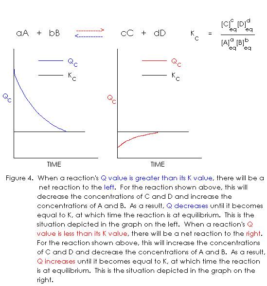
The analysis in Figure 4 shows how we can determine the direction of approach to equilibrium for any arbitrary starting concentrations. To illustrate the method of calculation, consider the following problem:
Into a 10.00 L reaction vessel, a chemist placed 0.381 moles of HI, 0.492 moles of H2, and 0.773 moles of I2 at 425 oC. the chemical equation for the equilibrium of HI, H2, and I2 is as follows:
2HI(g) <----------> H2(g) + I2(g) KC = 1.84 at 425 oC [Eq. 36]
Is this system at equilibrium? And if not, in which direction will the reaction proceed to reach equilibrium?
Solution:
We begin by obtaining the concentrations to plug into the QC expression. Both KC and QC are based on concentration in moles per liter. We have been given total moles, but since the volume is given also, we can calculate the concentrations:
[HI] = 0.381 mol / 10.00 L = 0.0381 M [Eq. 37]
[H2] = 0.492 mol / 10.00 L = 0.0492 M [Eq. 38]
[I2] = 0.773 mol / 10.00 L = 0.0773 M [Eq. 39]
Now we plug these concentrations into the QC expression to calculate a value for comparison with KC:
QC = [H2]t [I2]t / [HI]t2 = (0.0492) (0.0773) / (0.0381)2 = 2.62 [Eq. 40]
For this reaction at 425 oC, KC has a value of 1.84, but existing concentrations give a QC value of 2.62. Therefore, QC > KC so the system is not at equilibrium and reaction will take place to the left. That is, there will be a net conversion of H2 and I2 into HI until equilibrium is reached.
A couple of notes are worth mentioning about the problem just worked. First, in this particular case, we could have just used the total moles rather than calculating the concentrations, because the sum of the coefficients is the same on both sides of the equation. There is only one substance on the left side (HI) and it has a coefficient of 2. On the right side, there are two substances (H2 and I2), each with a coefficient of 1, giving a total of 2. When the sum of the coefficients is the same on both sides of the equation, the volume just cancels out in the QC expression. If we use the total moles in the QC calculation (equation 40) we will get the same QC value (2.62) that was obtained using the molar concentrations. However, anyone who wants to use this shortcut needs to be sure the sum of the coefficients is the same on both sides of the equation. That’s the only time it works. When in doubt, it is best to just use the concentrations – you can’t go wrong that way. Another point that should be made is that even though the concentrations have units of moles per liter (abbreviated as M for “molarity”), these units were not carried in the QC calculation. This was not an error. QC is supposed to be a dimensionless quantity. So even though we must make sure the numbers used in the calculation are in moles per liter, we don’t actually carry those units in the calculation. Actually, we should be using activities instead of concentrations in equilibrium calculations, and activities have no units. At low concentrations, the concentration and the activity are almost the same. They begin to deviate as the concentration becomes larger. In all the problems we work in General Chemistry II, our approach will be to assume that we can use concentrations in place of activities. This is the reason the units were dropped from the QC calculation.
4.4 Finding an Equilibrium Composition
In section 4.3, we learned about the reaction quotient QC and how it can be used, in conjunction with a KC value, to determine in which direction a reaction will proceed to reach equilibrium. Another useful calculation the equilibrium constant makes possible is the equilibrium composition. To illustrate this, let’s use the problem we worked on in the preceding section. We were given the following information:
2HI(g) <----------> H2(g) + I2(g) KC = 1.84 at 425 oC [Eq. 36]
And we had these starting concentrations:
[HI] = 0.381 mol / 10.00 L = 0.0381 M [Eq. 37]
[H2] = 0.492 mol / 10.00 L = 0.0492 M [Eq. 38]
[I2] = 0.773 mol / 10.00 L = 0.0773 M [Eq. 39]
We have already determined that the reaction will take place to the left, meaning some of the H2 and I2 will be used, and additional HI will be formed. The question is, what will all of these concentrations be when the system has reached equilibrium? We can answer this question by setting up a table that shows the starting concentrations, their relative changes, and the equilibrium values. Of course, since we don’t know what those values are, there will be an unknown variable X in our table. The equilibrium constant will allow us to solve for X. Your author likes to call these tables “ICE” tables, where the letters stand for Initial, Change, and Equilibrium. Here is what the ICE table looks like for this problem:
2HI(g) <----------> H2(g) + I2(g)
|
|
[HI] |
[H2] |
[I2] |
|
Initial |
0.0381 |
0.0492 |
0.0773 |
|
Change |
+2X |
-X |
-X |
|
Equilibrium |
0.0381 + 2X |
0.0492 – X |
0.0773 - X |
Here is how the table is filled out:
First, in the row labeled Initial, we fill in the starting concentrations for HI, H2 and I2. Since we know (from our earlier QC calculation) that the reaction is going to the left, we know that the H2 and I2 concentrations will be decreasing while the HI concentration will be increasing. Now look at the stoichiometry of the reaction. The H2 and I2 both have coefficients of 1, so they must decrease by equal amounts. The HI has a coefficient of 2, so its concentration will increase twice as fast as the H2 and I2 concentrations decrease. If we let X represent the amount by which the H2 and I2 concentrations decrease, then the HI concentration must increase by 2X. The X has a minus sign in front of it for H2 and I2 because those concentrations are decreasing, whereas the 2X that appears in the HI column has a positive sign in front of it (understood and not shown). Thus, the 2X, -X, and -X are the relative changes in concentration for HI, H2 and I2, respectively. To get the equilibrium concentrations, we add the initial concentrations and the concentration changes. This gives the expressions which are seen on the equilibrium row. At this point, we still don’t know what the equilibrium concentrations are, because they are given in terms of X, and we don’t know the numerical value of X. However, if these are equilibrium concentrations, they must satisfy the equilibrium constant expression for the reaction.
[H2]eq [I2]eq / [HI]2eq = KC [Eq. 40]
Substituting the concentrations from the ICE table into equation 40 gives
(0.0492 - X) ( 0.0773 - X) / (0.0381 + 2X)2 = 1.84 [Eq. 41]
This equation can be solved for X, and the value of X can be substituted into the ICE table to obtain the equilibrium concentrations. Equation 41 is readily solvable, but it is not exactly what we would call student friendly. The equation must be re-arranged into the standard form of a quadratic equation, which is then solved using the quadratic formula. The standard quadratic equation has the form
aX2 + bX + c = 0 [Eq. 42]
for which the solutions are given by
X = ( -b ± Ö ( b2 - 4ac ) ) / 2a [Eq.
43]
Rearranging Equation 41 into a form like Equation 42
yields the following:
6.36X2
+ 0.407X - 0.00113 = 0 [Eq.
44]
Comparing equations 42 and 44, we see that
A = 6.36,
b = 0.407 and c
= -0.00113 {Eq. 45]
Notice that a quadratic equation has two roots. This is reflected in the fact that the
square root can be either added or subtracted in Equation 43. When the mathematical solution to a physical
problem has more than one root, only one of the roots is physically
meaningful. There can be only one
equilibrium composition, not two or more.
In the present problem, we take the positive value of the square
root. The variable X has been defined
as the extent of reaction to the left; the value of X is subtracted from the
initial concentration of H2 and I2 and twice its value is
added to the initial concentration of HI.
If we calculate X using the negative value of the square root, we get a
negative value for X, which would imply that the H2 and I2
concentrations are increasing while the HI concentration is decreasing. This would be in conflict with the direction
of reaction obtained from our earlier QC calculation. Moreover, the magnitude of the negative root
(-0.0667)
would imply a greater extent of reaction than the available concentrations
would allow. The equilibrium
concentration of HI would be negative using this value of X. Therefore, we use the positive value of the
square root and obtain a value of 0.0027 for X. We can now substitute this value back into the ICE table to
obtain the equilibrium concentrations.
2HI(g) <----------> H2(g) + I2(g)
|
|
[HI] |
[H2] |
[I2] |
|
Initial |
0.0381 |
0.0492 |
0.0773 |
|
Change |
+0.0054 |
-0.0027 |
-0.0027 |
|
Equilibrium |
0.0435 |
0.0465 |
0.0746 |
We now have all the equilibrium concentrations. We can check to be sure this is an equilibrium set of concentrations by plugging them into a QC calculation and noting whither or not QC = KC.
QC
= [H2] [I2]
/ [HI]2 = (0.0465) (0.0746) / (0.0435)2 =
1.83 » 1.84
Our original data in this problem was only given to 3 significant figures, so we can accept 1.83 as being close enough to 1.84 to verify that this is an equilibrium set of concentrations.